Being able to work with common units is an essential skill for any scientist. They are integral to the way we measure physical quantities. This page covers the basic units and how to work with them. For a more detailed overview, see Chemistry Skills Hub. This page requires knowledge of powers and how to solve simultaneous equations, so if you're not sure on these skills, see our page on exponentials, and our page on simultaneous equations.

]]>

There are lots of different systems of units, such as the imperial system which uses pounds, feet and inches, or the metric system which uses kilograms, metres and litres. The one most widely used by scientists is the International System of Units (or SI for short, from the French "Système international d'unités").The SI system is based on seven basic units, and all other units of measurement are derived from these. These seven units are:

Kilogram (kg), for mass
Metre (m), for length
Ampere (A), for electric current
Kelvin (K), for temperature
Second (s), for time
Candela (cd), for luminous intensity
Mole (mol), for amount of a substance

Image showing basic units. The units shown are kilogram (kg) for mass, meter (m) for length, ampere (A) for electric current, kelvin (K) for temperature, second (s) for time, candela (cd) for luminous intensity and mole (mol) for amount of substance. — Image developed by the UoY Department of Biology

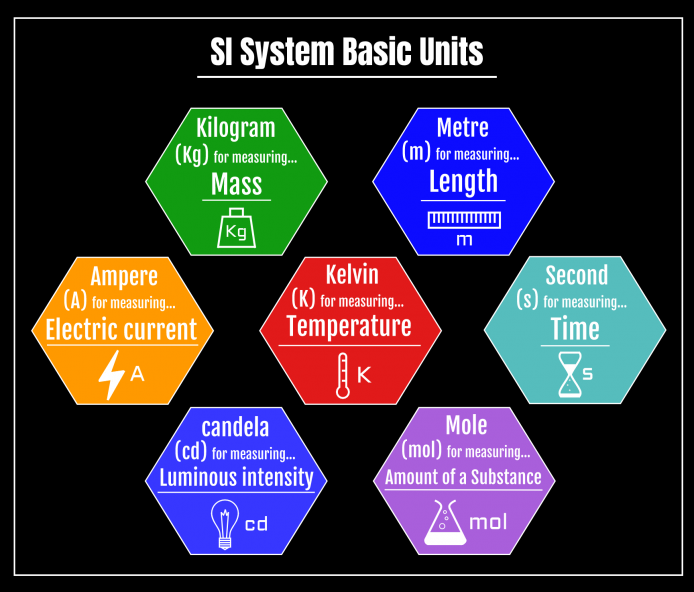
Another common unit to measure molecular mass is the Dalton (Da), which is defined as the mass of one hydrogen atom. This is commonly used in biology to describe the masses of amino acids and proteins. For example a protein with a molecular weight of 36,000 g mol^-1, has a mass of 36,000 daltons, or 36 kDa.We also have other units that are defined in terms of these basic units, such as:

Metres per second (m/s, ms^-1) for speed
Metres per second per second (m/s², ms^-2) for acceleration
Pascals (Pa) for pressure, defined as the force of 1 N acting on an area of 1 m²
Joules (J) for energy, defined as the work done by 1 N acting over a distance of 1 m.

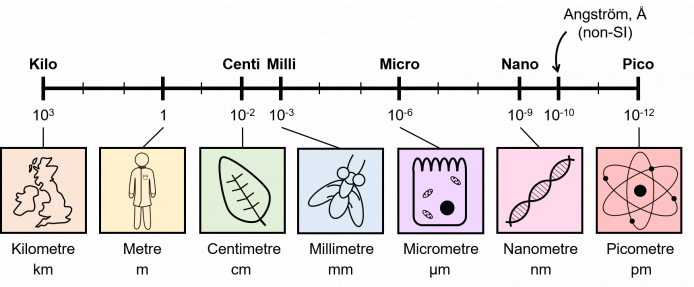
We can often work out what the units for a physical quantity are by looking at the at the equation to calculate them. For example, speed is calculated as:\[\text{speed} = \frac{\text{distance}}{\text{time}} \sim \frac{\text{metres}}{\text{seconds}}\]So the units for speed are metres divided by seconds, or m/s. We could also write it as metres multiplied by seconds^-1, or ms^-1. We pronounce m/s, as metres per second. In general, whenever you see a "/" in a unit, you can replace it with "per".Similarly, we can calculate acceleration:\[\text{acceleration} = \frac{\text{speed}}{\text{time}} = \frac{\frac{\text{distance}}{\text{time}}}{\text{time}} = \frac{\text{distance}}{\text{time}^2} \sim \frac{\text{metres}}{\text{seconds}^2}\]Hence, acceleration is measured in metres divided by seconds², or m/s². Again, we could write it as metres multiplied by seconds^-2, or ms^-2. Or we could just say metres per second², or metres per second per second.We often want to measure quantities that would give really big or really small numbers if we used the standard units for that quantity. Therefore it's convenient to have a system of prefixes that defines units of different orders of magnitude of the same unit, such as millimetres, centimetres, metres, kilometres etc.

Image showing differences in sized items between picometers all the way through to kilometers. — Image developed by the UoY Department of Biology

Overview of SI prefixes
Prefix	Multiplied by	Symbol
exa	$10^{18}$	E
peta	$10^{15}$	P
tera	$10^{12}$	T
giga	$10^{9}$	G
mega	$10^6$	M
kilo	$10^3$	k
hecto	$10^2$	h
deca	$10$	dk
deci	$10^{-1}$	d
centi	$10^{-2}$	c
milli	$10^{-3}$	m
micro	$10^{-6}$	$\mu$
nano	$10^{-9}$	n
pico	$10^{-12}$	p
femto	$10^{-15}$	f
atto	$10^{-18}$	a

The table above shows the standard SI prefixes, along with the factor that you have to multiply the standard units by, and their symbols. For example, there are $10^9$ metres in a gigametre, and a gigametre is denoted by Gm.To move up the table, you normally divide by $10^3(=1000)$, and to move down the table you normally multiply by $10^3(=1000)$. For example, to convert millimetres to metres, you divide by $1000$, and to convert metres back to millimetres, you multiply by $1000$. Note: This rule doesn't work to convert between hecto, deca, deci, or centi.

]]>

We can express physical quantities in terms of their dimensions. Most physical quantities can be expressed in terms of these basic dimensions:

Mass (M)
Length (L)
Time (T)
Electrical current (l)
Temperature ($\theta$)

Dimensions are not the same as units, for example we can measure speed in metres per second, kilometres per hour, or miles per hour; but it is always a length divided by a time regardless of the units, so the dimensions of speed are L/T.Similarly, we can measure area as square metres, or square kilometres, or square miles, but it is always a length squared, so the dimensions of area are L².We can use this to work out the units of a constant or variable in an equation, by substituting the dimensions of the variables into the equation. This is based on the principle of consistency of dimensions, if two expressions are equal, their dimensions must be the same.Notation: To denote the dimensions of a physical quantity $X$, we use square brackets, $[X]$.

]]>Assuming that force is proportional to the square of speed, i.e.,\[\color{blue}F=k\color{red}v^2\]for some constant $k$. Find the dimensions of $k$.

We know that force is mass times acceleration, $F = ma$, so we can write the dimensions of force as $\color{blue}{[F] = [m][a] = M L T^{-2}}$ since acceleration is a length divided by a time squared. We also have the dimensions of speed as a length over a time, $\color{red}{[v] = L/T = LT^{-1}}$.

So now we can put this into our original equation:\[\color{blue}{MLT^{-2}} =[k](\color{red}{LT^{-1}})^2 = [k]L^2T^{-2}\]Now we rearrange to find $[k]$.\[\begin{align} [k] &= \frac{MLT^{-2}}{L^2T^{-2}} \\ &= \frac{ML}{L^2}\\ &=\frac{M}L \end{align}\]So we now that $k$ is a mass divided by a length, or we can measure it in terms of kg/m.

]]>We can also write force ($\color{blue}F$) in terms of radius ($\color{red}r$), length ($\color{green}l$), speed ($\color{purple}v$), distance ($\color{orange}R$) and viscosity ($\eta$):\[\color{blue}F = -2\pi \color{red}r\color{green}l\frac{\color{purple}v}{\color{orange}R}\eta\]Find the dimensions of viscosity ($\eta$) using dimensional analysis.

It's helpful to write down all the dimensions we know:

Force is $\color{blue}{MLT^{-2}}$.
Radius is a length, $\color{red}L$.
Length is a length, $\color{green}L$.
Speed is a length divided by a time, $\color{purple}{LT^{-1}}$.
Distance is a length, $\color{orange}L$.

We can now substitute all of these into the equation, noting that we can ignore the dimensions of $-2\pi$ since that's just a number that has no dimensions.\[\begin{align} \color{blue}{MLT^{-2}} &= \color{red}L \color{green}L \frac{\color{purple}{LT^{-1}}}{\color{orange}L}[\eta] \\ &= L^2T^{-1}[\eta] \\ MT^{-2} &= LT^{-1}[\eta] \\ L[\eta] &= MT^{-1} \\ [\eta] &= ML^{-1}T^{-1} \end{align}\]So we have that the dimensions of viscosity are a mass divided by a length and a time, so we can measure it in kgm^-1s^-1.

]]>We can use dimensions to find relationships between physical quantities. Assuming we can write one quantity in terms of a power of another quantity (up to a scaling constant) allows us to write an equation in terms of these quantities, $y = Cx^a$. We can then substitute in their dimensions ($[y] = [x]^a$) and compare the powers of the dimensions to find the relationship between the quantities. This is easier to see with an example - see below.If you're interested: We can assume the relationship is a power function, $y = Cx^a$, because these functions are the only functions whose form does not alter when we re-scale the variables. This is important because the units that we choose as scientists shouldn't affect the form of the relationship between $x$ and $y$, so if you believe that a physical law takes the same form regardless of the units, then it must take the form of a power law.

]]>The maximum speed $v$ of a ship, however large its engines, depends only on its length $l$ and on the acceleration due to gravity $g$.

Suppose that $v$ is proportional to some power of $l$, that \[v \propto l^a\]Use dimensional arguments to find $a$.

Since $v$ depends on $l$ and $g$, we can write\[v = Cl^a g^b\]for some dimensionless constant $C$. Now taking dimensions gives us\[LT^{-1} = L^a(LT^{-2})^b = L^{a + b}T^{-2b}\]since $g$ is an acceleration due to gravity. Matching the dimensions yields\[1 = a+ b \\ -1 = -2b\]which can be solved to give\[b = \frac12 \\ a = \frac12\](So this gives $v \propto \sqrt{gl}$.)

]]>You wish to know the time taken ($t$) to cook a turkey of mass $m$. Suppose that $t$ depends on $m$, on the density $\rho$ of the meat, and on the thermal diffusivity $\kappa$, whose dimensions are $L^2T^{-1}$ . Find the dependence of $t$ on $m$, $\rho$, $\kappa$ in the form \[t = Cm^a\rho^b\kappa^c\]where $C$ is a dimensionless constant.

Taking dimensions of the equation gives us\[T = M^a(ML^{-3})^b(L^2T^{-1})^c = M^{a+b}L^{-3b+2c}T^{-c}\]which yields the equations\[1 = -c \\ 0 = a + b \\ 0 = -3b+2c\]Solving these simultaneously gives us\[a = \frac23 \\ b =-\frac23 \\ c = -1\]So then\[t = Cm^{\frac23}\rho^{-\frac23}\kappa^{-1} \propto m^{\frac23}\rho^{-\frac23}\kappa^{-1}\]

]]>

Which one of the following expressions are correct for the mean speed of molecules in the ideal gas?

\[\sqrt{\frac{3RT}{M}}\]
\[\sqrt{\frac{M}{3RT}}\]

]]>Look at the units of the two expressions.

]]>The left hand side has the units of $ms^{-1}$. The right hand side of (1) has the units of\[\sqrt{\frac{\text{J }\text{mol}^{-1}\text{K}^{-1}\text{K}}{\text{kg mol}^{-1}}} = \sqrt{\frac{\text{J}}{\text{kg}}} = \sqrt{\frac{\text{kg m}^2\text{s}^{-2}}{\text{kg}}} = \sqrt{\text{m}^2\text{s}^{-2}} = \text{ms}^{-1}\]and the right hand side of (2) has the units of \[\sqrt{\frac{\text{kg mol}^{-1}}{\text{J }\text{mol}^{-1}\text{K}^{-1}\text{K}}} = \sqrt{\frac{\text{kg}}{\text{J}}} = \sqrt{\frac{\text{kg}}{\text{kg m}^2\text{s}^{-2}}} = \sqrt{\text{m}^{-2}\text{s}^2} = \text{m}^{-1}\text{s}\]So the units of (2) don't match, so (1) is correct.

]]>Efficient deposition of respiratory drugs through inhalers requires the patients to breathe deeply and to hold their breath for a while. The powder of density $\rho$, consisting of drug particles of diameter $d$ fall through the air and reach the terminal velocity (speed) $v$ determined by the balance between gravity (gravitational acceleration, $g$) and the viscosity of the air $\eta$ (kg m^-1s^-1).

Based on the observation that the terminal velocity $v$ is proportional to the powder density, express $v$ in terms of $\rho$, $g$, $d$, and $\eta$ using dimensional analysis.

]]>Since $v$ is proportional to $\rho$, let us first assume\[v=\Gamma \rho g^xd^y\eta^z\]where $\Gamma$ is a unitless constant. Let us match the dimensions between the left and right hand sides. On the left, we have $LT^{-1}$. On the right, we have\[ML^{-3}(LT^{-2})^x L^y (ML^{-1}T^{-1})^z = M^{1+z}L^{x+y+z-3}T^{-2x-z}\]

So now we have\[LT^{-1}= M^{1+z}L^{x+y+z-3}T^{-2x-z}\]

Matching the LHS and RHS dimensions yields\[z=-1 \\ x+ y - z - 3 = 1 \\ -2x+1 = -1\]Solving the simultaneous equations yields\[x=1 \\y=2\\z=-1\]
Thus we obtain \[v = \Gamma\rho g d^2\eta^{-1}\]

]]>To create blood flow, the vascular resistance $R$ (Pa m^-3s) must be overcome by the heart.

Experiments show that $R$ is proportional to the length of the blood vessel $L$ (m). Use dimensional analysis to show that $R$ is expressed in terms of $L$, the viscosity of blood (Pa s), and the radius of the blood vessel $r$ (m) in the following form:

\[R = \Gamma \frac{L\eta}{r^4}\]

where $\Gamma$ is a dimensionless constant.

]]>Using the fact that $R$ is proportional to $L$, we can start from the following relationship relating $R$ to $L$,$\eta$, and $r$:
\[R = \Gamma L \eta^xr^y\]
where $\Gamma$ is a unit-less constant. The dimensions are
Left hand side: \[[\text{Pa}] L^{-3}T= ML^{-1}T^{-2}L^{-3}T = ML^{-4}T^{-1}\]
Right hand side: \[L([\text{Pa}]T)^xL^y = L(ML^{-1}T^{-1})^xL^y = L^{1-x+y}M^xT^{-x}\]Consistency of units requires
\[x=1 \\1-x+y=-4\]
Solving the simultaneous equations yields
\[x=1\\y=-4\]
Thus we obtain
\[R=\Gamma L\eta r^{-4} = \Gamma\frac{L\eta}{r^4}\]

]]>

Which one of the following expressions are correct for the mean speed of molecules in the ideal gas?

\[\sqrt{\frac{3RT}{M}}\]
\[\sqrt{\frac{M}{3RT}}\]

]]>Look at the units of the two expressions.

]]>Electrophoresis is used routinely in biochemical laboratories as one of the first recourse to see what molecules are there in the sample.

Charged molecules (each with charge $q$ [C=coulomb]) travel through the electric field $E$ (N C^-1). Each molecules experience frictional drag $f$ (N s m^-1).

Calculate the speed $v$ of the molecule.

]]>Improvising an equation, we can write\[v= \Gamma q^xE^yf^z\]where $\Gamma$ is a unitless constant. The units on the left hand side are m s^-1, and the units on the right hand side are\[\text{C}^x(\text{NC}^{-1})^y (\text{N s m}^{-1})^z = \text{C}^{x-y} \text{N}^{y+z}\text{s}^z\text{m}^{-z}\]Matching units, we have\[\text{ms}^{-1} = \text{C}^{x-y} \text{N}^{y+z}\text{s}^z\text{m}^{-z}\]which gives us\[x - y = 0 \\ y + z = 0 \\ z = -1\]solving these simultaneously, gives us\[x = 1 \\ y=1\\ z=-1\]So then\[v = \Gamma q E f^{-1} = \Gamma \frac{qE}{f}\]

]]>Time-of-flight mass spectrometer determines the mass-to-charge ratio of an ion based on the time taken to reach the detector located at a known distance. The ion flies through the electric field to the detector.

(a) Express the flight time $t$ (s) in terms of mass of the ion $m$ (kg), charge of the ion $q$ (C = coulomb), the electrostatic potential $\varepsilon$ (J C^-1), and the length of flight $L$.

(b) Express the speed of the ion $v$ in terms of the mass $m$, charge $q$ and the electrostatic potential $\varepsilon$.

]]>(a) We can write \[t = \Gamma m^x q^y \varepsilon ^z L^w\]where $\Gamma$ is a unitless constant. The units of the left hand side are s, and the units of the right hand side are\[\begin{align} \text{kg}^x\text{C}^y (\text{J C}^{-1})^z \text{m}^w &= \text{kg}^x\text{C}^y(\text{kg m}^2 \text{s}^{-2}\text{C}^{-1})^z \text{m}^w \\ &= \text{kg}^{x+z}\text{C}^{y-z}\text{m}^{2z+w}\text{s}^{-2z} \end{align}\]Comparing units gives us\[x+z = 0 \\ y-z=0 \\ 2z+w = 0 \\ -2z=1\]Solving these simultaneously yields\[x = \frac12\\ y = -\frac12\\ z = -\frac12\\ w = 1\]So now we have\[t = \Gamma m^{\frac12}q^{-\frac12}\varepsilon^{-\frac12}L = \Gamma \sqrt{\frac{m}{q\varepsilon}}L\](b) We can calculate the speed of the ion by simply dividing the length of flight $L$, by the flight time, $t$. So\[v = \frac{L}{\Gamma \sqrt{\frac{m}{q\varepsilon}}L} = \frac1{\Gamma}\sqrt{\frac{q\varepsilon}{m}}\](c) We can check our answer by considering the units of the above, which should be m s^-1 since it's a speed. The units of the right hand side are\[\sqrt{\frac{\text{CJC}^{-1}}{\text{kg}}} = \sqrt{\frac{\text{J}}{\text{kg}}} = \sqrt{\frac{\text{kg m}^2\text{s}^{-2}}{\text{kg}}} = \sqrt{\text{m}^2\text{s}^{-2}} = \text{m s}^{-1}\]So our answer makes sense.

]]>

Show that energy density (measured in J/m³) is equal to pressure (measured in Pa).

]]>First, we need to remember that energy is the same as work done, which is force times distance. So we can write\[\text{Energy density} = \frac{\text{Energy}}{\text{Volume}} \sim \frac{\text{J}}{\text{m}^3} = \frac{\text{Nm}}{\text{m}^{3}} = \frac{\text{N}}{\text{m}^2} = \text{Nm}^{-2}\]and since the units of pressure are Pascals, or Nm^-2, this shows that energy density is the same as pressure.

]]>Return to Subject Applications

]]>

Producing a straight line is useful not only for determining thermodynamic and kinetic parameters by linear linear regression but also for showing (persuading) that a model of thermodynamics (such as van’t Hoff equation) or kinetics (such as the first and second order kinetics) applies to your experimental data.

The exercises below will train you all the mathematical skills required to understand and practice linearisation.

]]>

These questions will help you translate your understanding of the pure maths techniques to applied questions. Feel free to skip questions, but if you are struggling with the more applied questions, go back and look at earlier exercises to help build your understanding and confidence.

These exercises will use logarithms, if you need a refresher before you attempt these problems, we encourage you to look at the Exponentials and Logarithms section of the Maths Survival Skills webpage.

]]>Linearise \[y=2e^{-3x}\]And sketch the linearised graph

Take the natural logarithm on both sides,\[\ln(y)=\ln(2e^{-3x})\]Then simplify\[\ln(y)=\ln(2) -3x\]Now we can sketch a linear graph using

$x$ is the horizontal axis
$\ln(y)$ on the vertical axis
$\ln(2)$ as the y-intercept
$-3$ is the gradient

]]>

A graph of a straight line with ln(y) on the vertical axis and the y intercept labelled as ln(2)

Linearise \[y=2e^{\frac{3}{x}}\]And sketch the linearised graph

Important note: If you use $x$ as the independent variable, you don’t get a linear plot. You have to use $\frac{1}{x}$.

]]>Linearise \[y=2e^{\frac{3}{x}}\]And sketch the linearised graph

Take the natural logarithm on both sides,\[\ln(y)=\ln(2e^{\frac{3}{x}})\]Then simplify\[\ln(y)=\ln(2) +3\frac{1}{x}\]Now we can sketch a linear graph using

$\ln(y)$ on the vertical axis
$\frac{1}{x}$ on the horizontal axis
$\ln(2)$ as the y-intercept
$3$ is the gradient

]]>

A graph of a straight line with ln(y) on the vertical axis, 1/x on the x axis and the y intercept labelled as ln(2)

The Arrhenius equation connects the rate constant $k$ to the activation energy $E_a$ and the pre-exponential factor $A$.

Linearise \[k=Ae^{-\frac{E_a}{RT}}\]And sketch the linearised graph

You change $T$ and measure $k$ experimentally. $E_a$ is the activation energy you want to get from the Arrhenius equation.

]]>The Arrhenius equation connects the rate constant $k$ to the activation energy $E_a$ and the pre-exponential factor $A$.

Linearise \[k=Ae^{-\frac{E_a}{RT}}\]

And sketch the linearised graph

You change $T$ and measure $k$ experimentally. $E_a$ is the activation energy you want to get from the Arrhenius equation.

$k$: rate constant, $R$: gas constant, $E_a$: activation energy, $A$: pre-exponential factor (representing, for example, collision), $T$: temperature.

This exercise is similar to Exercise 2, as x is called T and 3 is now $\frac{E_a}{R}$

Take the natural logarithm on both sides,

\[\ln(k)=\ln\left(Ae^{-\frac{E_a}{RT}}\right)\]Then simplify\[\ln(k)=\ln\left(A\right) -\frac{E_a}{R}\frac{1}{T}\]Now we can sketch a linear graph using

$\ln(k)$ on the vertical axis
$\frac{1}{T}$ on the horizontal axis
$\ln(A)$ as the y-intercept
$-\frac{E_a}{R}$ is the gradient

]]>

A graph of a straight line with ln(k) on the vertical axis, 1/T on the x axis and the y intercept labelled as ln(A)

When $x$ is the independent variable, linearise\[xy=2-3x\]And sketch the graph

]]>When $x$ is the independent variable, linearise\[xy=2-3x\]And sketch the graph

Divide both sides by $x$
\[y = 2\frac{1}{x}-3\]Now we can sketch a linear graph using

y on the vertical axis
$\frac{1}{x}$ on the horizontal axis
$-3$ as the y-intercept
$2$ is the gradient

This looks like a very strange question. But you will see the same approach will be used in Exercise 5

]]>

A graph of a straight line with 1/x on the x axis

When $\Delta H$ and $\Delta S$ are constants, linearise \[-RT\ln(K) = \Delta H- T\Delta S\]And sketch the linearised graph.

$\Delta H$ and $\Delta S$ are constants, but $K$ changes with $T$.

]]>Linearise \[-RT\ln(K) = \Delta H- T\Delta S\]

And sketch the linearised graph

where $\Delta H$ and $\Delta S$ are constants, but K changes with T

This exercise is similar to Exercise 4.

Divide both sides by T
\[-R\ln(K) = \Delta H\frac{1}{T}- \Delta S\]Now we can sketch a linear graph using

$-R\ln(K)$ on the vertical axis
$\frac{1}{T}$ on the horizontal axis
$-\Delta S$ as the y-intercept
$\Delta H$ is the gradient

]]>

A graph of a straight line with -Rln(k) on y axis, 1/T on the x axis and - delta s as the intercept

This is referred to as a van't Hoff plot.

Experimentally, measure $K$ at different temperatures. Plotting them on a van’t Hoff plot will give you $\Delta H$ and $\Delta S$ if neither of them change with temperature.

]]>Linearise \[y=\frac{1}{2x+5}\]And sketch the linearised graph

Divide both sides by y and then multiply both sides by 2x+5
\[\frac{1}{y} = 2x+5\]Now we can sketch a linear graph using

$\frac{1}{y}$ on the vertical axis
x on the horizontal axis
$5$ as the y-intercept
$2$ is the gradient

]]>

A graph of a straight line with 1/y on the y axis

Linearise \[[A]=\frac{1}{kt+\frac{1}{[A]_0}}\]where t is time, k is the rate constant, $[A]$ is the concentration of the chemical species A and $[A]_0$ is the initial concentration of A.

Sketch the linearised graph

]]>Linearise \[[A]=\frac{1}{kt+\frac{1}{[A]_0}}\]where t is time, k is the rate constant, $[A]$ is the concentration of the chemical species A and $[A]_0$ is the initial concentration of A.

Sketch the linearised graph

This exercise is similar to Exercise 6.

Rearranging gives
\[\frac{1}{[A]}=kt+\frac{1}{[A]_0}\]Now we can sketch a linear graph using

$\frac{1}{[A]}$ on the vertical axis
t on the horizontal axis
$\frac{1}{[A]_0}$ as the y-intercept
$k$ is the gradient

This is the linearised plot for the second-order rate equation.

]]>

A graph of a straight line with 1/[A] on the y axis, t on the x axis, 1/[A]_0 as the intercept

Return to Subject Applications

]]>

A (bio)chemical reaction is characterised by the equilibrium constant $K$. The major goal of (bio)chemical thermodynamics for chemists and biochemists is to understand $K$ on a molecular basis. This requires you to convert $K$ to $\Delta G$, so that you can compare it with the heat of reaction and entropy. Studying thermodynamics means going back and forth between $K$ and $\Delta G$.

The exercises below will use logarithms. If you need a refresher before you attempt these problems, we encourage you to look at the Exponentials and Logarithms section of the Maths 'Survival' Skills webpage.

]]>

]]>Find the simplest expression for $\ln(y)$\[y=e^{-x}\]

Solution

Take the natural logarithm on both sides\[\ln(y)=\ln(e^{-x})\]Then simplify

\[\ln(y)=-x\]

]]>Find the simplest expression for $\ln(y)$\[y=e^{-2x}\]

Solution

Take the natural logarithm on both sides\[\ln(y)=\ln(e^{-2x})\]Then simplify

\[\ln(y)=-2x\]

]]>Find the simplest expression for $\ln(y)$\[y=e^{-\frac{x}{2}}\]

Solution

Take the natural logarithm on both sides\[\ln(y)=\ln(e^{-\frac{x}{2}})\]Then simplify

\[\ln(y)=-\frac{x}{2}\]

]]>Find the simplest expression for $\ln(y)$\[y=\frac{e^{-x}}{2}\]

Solution

Take the natural logarithm on both sides\[\ln(y)=\ln\left(\frac{e^{-x}}{2}\right)\]Then simplify\[\ln(y)=\ln(e^{-x})-\ln(2)\]

\[\ln(y)=-x-\ln(2)\]

]]>Find the simplest expression for $\ln(y)$\[y=\frac{3}{2}e^{-x}\]

Solution

Take the natural logarithm on both sides\[\ln(y)=\ln\left(\frac{3}{2}e^{-x}\right)\]Then simplify\[\ln(y)=\ln(e^{-x})+\ln(\frac{3}{2})\]

\[\ln(y)=-x+\ln(\frac{3}{2})\]

]]>Find the simplest expression for $\ln(y)$\[y=e^{-\frac{E}{RT}}\]

Solution

This question is very similar to the one in Exercise 3, think of E as x and RT as 2 in that instance.

Take the natural logarithm on both sides\[\ln(y)=\ln(e^{-\frac{E}{RT}})\]Then simplify

\[\ln(y)=-\frac{E}{RT}\]

]]>Find the simplest expression for $\ln(y)$\[y=g(E)e^{-\frac{E}{RT}}\]

Solution

This question is similar to Exercise 5 where g(E) acts the same way as $\frac{3}{2}$.

Take the natural logarithm on both sides\[\ln(y)=\ln(g(E)e^{-\frac{E}{RT}})\]Then simplify\[\ln(y)=\ln(e^{-\frac{E}{RT}})+\ln(g(E))\]

\[\ln(y)=-\frac{E}{RT} +\ln(g(E))\]

]]>Find the simplest expression for $\ln(K)$\[K=e^{-\frac{\Delta H}{RT}}\](Where $\Delta H$ is enthalpy change)

Solution

This question still uses the same technique as all the previous parts, we have just replaced $y$ with $K$.

Take the natural logarithm on both sides\[\ln(K)=\ln(e^{-\frac{\Delta H}{RT}})\]Then simplify

\[\ln(K)=-\frac{\Delta H}{RT}\]

]]>Find the simplest expression for $\ln(K)$\[K=\frac{W_f}{W_i}e^{-\frac{\Delta H}{RT}}\]Where $\Delta H$ is enthalpy change, $\Delta H = H_f-H_i$, $W_i $ and $W_f$ are the number of configurations of the initial and final states respectively

Solution

This exercise is similar to Exercise 5 and 7, go back and have a look at them if you are struggling with this question.

Take the natural logarithm on both sides\[\ln(K)=\ln\left(\frac{W_f}{W_i}e^{-\frac{\Delta H}{RT}}\right)\]Then simplify\[\ln(K)=\ln\left(e^{-\frac{\Delta H}{RT}}\right)+ \ln\left(\frac{W_f}{W_i}\right)\]

\[\ln(K)=-\frac{\Delta H}{RT}+ \ln\left(\frac{W_f}{W_i}\right)\]This equation shows the important contributions for the equilibrium constant. The enthalpy gap $\Delta H$ and the numbers of initial and final states.

]]>Given that\[K=\frac{W_f}{W_i}e^{-\frac{\Delta H}{RT}}\]Show that \[-RT\ln(K) = \Delta H- T\Delta S\]Where $\Delta S = R\ln\left(\frac{W_f}{W_i} \right)$

Where $\Delta H$ is enthalpy change, $\Delta H = H_f-H_i$, $W_i $ and $W_f$ are the number of configurations of the initial and final states respectively and $\Delta S$ is entropy change.

]]>Given that\[K=\frac{W_f}{W_i}e^{-\frac{\Delta H}{RT}}\]Show that \[-RT\ln(K) = \Delta H- T\Delta S\]Where $\Delta S = R\ln\left(\frac{W_f}{W_i} \right)$

Where $\Delta H$ is enthalpy change, $\Delta H = H_f-H_i$, $W_i $ and $W_f$ are the number of configurations of the initial and final states respectively and $\Delta S$ is entropy change.

Solution

\[\ln(K)=-\frac{\Delta H}{RT}+ \ln\left(\frac{W_f}{W_i}\right)\]Multiply both sides by $RT$ \[-RT\ln(K)=\Delta H-RT \color{blue}{\ln\left(\frac{W_f}{W_i}\right)}\]Rearrange the equation for $\Delta S$ and substitute it in\[\color{blue}{\frac{\Delta S}{R} = \ln\left(\frac{W_f}{W_i} \right)}\]\[-RT\ln(K)=\Delta H-RT \color{blue}{\frac{\Delta S}{R}}\]Cancel out R from the last term to obtain the final answer\[-RT\ln(K) = \Delta H- T\Delta S\]This is a very important equation relating the equilibrium constant to the Gibbs free energy \[\Delta G \equiv \Delta H – T \Delta S\]

]]>

Return to Subject Applications

]]>

Presenting your experimental data as a graph is an excellent way to visualise your results and identify trends in your data. A well-designed graph will enable the reader to easily understand your results and readily comprehend the information you are trying to convey. We normally plot the independent variable on the $x$-axis and the dependent variable on the $y$-axis. The independent (or controlled) variable is the variable that the experimenter changes in a defined, incremental way (e.g. time). The dependent (or measured) variable is the variable which is recorded by the experimenter (e.g. absorbance of a solution).When plotting data, we refer to it in a specific way so that the listener understands what the variables are in the data set. For example, a plot of “absorbance versus time” indicates the above situation where absorbance is plotted on the $y$-axis, and time is plotted on the $x$-axis.For any type of graph, you should also ensure that the axes are properly labelled, and don’t forget to include units of measurement (e.g. grams, centimetres, minutes, g/L, mM) in these labels where required. If you are plotting more than one set of data on a graph then use a different colour or type of symbol for each data series, and ensure all data have the same units of measurement before plotting them together. Ensure you also include a legend with clear labels for each data series.When labelling your axes, it's good practice to put the units of the quantity measured on the axis. Chemists and physicists will usually use a forward slash to denote this (e.g. quantity/units) whereas biologists and biochemists might use brackets instead (e.g. quantity (units)). This page showcases a mixture of these two conventions to emphasise that either one is fine, as long as you are consistent. Scaling of the axes in a graph should be adjusted so the data covers a good proportion of the available area. Appropriate axes scaling makes it easier to inspect the amount of scatter in your data and identify systematic trends. Axis numbering usually starts at zero unless there is a good reason not to adhere to this convention. For instance, if doing this would force the data to occupy just a small proportion of the area in the graph. Each axis should have a reasonable number of ticks, which are evenly spaced and include a suitable number of significant figures (e.g. 0.0, 0.1, 0.2, 0.3,... rather than 0.000, 0.086, 0.186, 0.286,…).

]]>

Different types of graphs are appropriate for different types of experimental data.Bar graph: Often used to compare average values for different trials or experimental groups. A good option if your independent variable is not numerical, e.g. days of the week.

Bar graph of number of ambulances called for each day of a week

Time series plot: Standard format for plotting data where your dependent variable is numerical and your independent variable is time. You may need to fit your data with an equation to quantify the rate at which the dependent variable changes in time.

Time series plot of the amount of product formed in a reaction vs time

XY scatter plot: Typical format for plotting data where dependent and independent variables are both numerical, and you want to show how two variables may be related to one another. You may need to fit your data with an equation to quantify the relationship between the two variables.

Scatter plot of the density of a material vs temperature

]]>

You are given a data set where the absorbance at 562 nm of solutions containing different amounts of purified protein (μg) were measured. How should a plot of absorbance at 562 nm vs amount of protein (μg) look?

Amount of protein ($\mu g$)	Absorbance at 562 nm
0	0.094
1.25	0.182
6.25	0.258
12.5	0.474
25	0.783
37.5	1.009
50	1.44
75	1.801

It’s not necessary to plot the data to answer this question, you simply have to write down what variables are plotted on the $x$ and $y$ axes.

]]>The independent variable here is the amount of purified protein in each solution, therefore the amount of protein (µg) should be plotted on the $x$-axis. The absorbance at 562 nm is the dependent variable and should be plotted on the $y$-axis. Please see the ‘Graphical answer’ tab for an example of how this data might be plotted.

]]>

Scatter plot of absorbance at 562 nm vs. amount of protein

]]>You monitor the growth of a bacterial culture by measuring the absorbance at 600 nm as a function of time. You are asked to analyse how the level of bacterial growth changes with time. How would you plot your data to visualise this relationship?

Time (min)	Absorbance at 600 nm
0	0.0561
70	0.135
102	0.329
160	1.168
192	2.64
225	3.62
260	4.54
290	5.12
325	6.2
360	6.5
395	6.76
440	6.94
490	7.06
560	7.24

It’s not necessary to plot the data to answer this question, you simply have to write down what variables are plotted on the $x$ and $y$ axes.

]]>The independent variable here is time (min), therefore this data should be plotted on the $x$-axis. The absorbance at 600 nm is the dependent variable and should be plotted on the $y$-axis. Please see the ‘Graphical answer’ tab for an example of how this data might be plotted.

]]>

Time series plot of absorbance at 600 nm vs. time

]]>You have measured the fractional saturation ([PL]/[P_total]) of a specific protein’s binding site at different concentrations of a specific ligand ([L]) and constant protein concentration ([P_total]). This data needs to be fit with the follow equation where $K_a$ is a constant:\[\frac{[\text{PL}]}{[\text{P}_\text{total}]} = \frac{K_a[\text{L}]}{1 + K_a[\text{L}]}\]How would you plot this data to facilitate the data fitting process?

It’s not necessary to plot the data to answer this question, you simply have to write down what variables are plotted on the $x$ and $y$ axes.

]]>The first step in answering this question is to identify which parameters in the equation are the independent and dependent variables, and which parameters in the equation are constant.

The independent variable here is the concentration of specific ligand ($[\text{L}]$), therefore this data should be plotted on the $x$-axis. The fractional saturation ($\text{[PL]}/[\text{P}_{\text{total}}]$) is the dependent variable that you have measured and should be plotted on the $y$-axis.

The other parameter in the equation is the equilibrium association constant ($K_a$) which is a constant. You want to determine a value for this parameter by fitting your plotted data with the following equation: \[\frac{\text{[PL]}}{[\text{P}_{\text{total}}]} = \frac{K_a\text{[L]}}{1 + K_a\text{[L]}}\]
(FYI: This data fitting could be done in R using non-linear regression). Please see the ‘Graphical answer’ tab for an example of how this data might be plotted.

]]> $Scatter plot of fractional saturation vs [L]$

]]>You are using absorption spectroscopy to monitor the reaction kinetics for hydrolysis of a chemical compound. You have generated time-dependent absorbance data (Abs_t) for the product of the reaction and want to fit this data with the following equation where $b$, $c$ and $k_{\text{obs}}$ are constants: \[\text{Abs}_t = b - ce^{-k_{\text{obs}}t}\]How would you plot this data to facilitate the data fitting process?

It’s not necessary to plot the data to answer this question, you simply have to write down what variables are plotted on the $x$ and $y$ axes.

]]>The first step in answering this question is to identify which parameters in the equation are the independent and dependent variables, and which parameters in the equation are constant.

The independent variable here is time in seconds, therefore this data should be plotted on the $x$-axis. You should not worry that the equation has the time variable ($=t$) in the exponential term. The absorbance at 405 nm is the dependent variable that you have measured to monitor progression of the reaction and should be plotted on the $y$-axis.

The other parameters in the equation are the $b$ and $c$ terms, and pseudo-first order rate constant ($k_{\text{obs}}$), all of which are constants. You want to determine a value for $k_{\text{obs}}$ by fitting your plotted data with the following equation: \[\text{Abs}_t = b - c e^{-k_\text{obs}t}\]
The parameters $b$ and $c$ define the asymptotic (at long time) and initial values of the measured absorbance at 405 nm, respectively. In the representative data plot provided here, they would have approximate values of $b=1 $ and $c = 0.8 $, which you would determine by fitting your data with the above equation (FYI: This data fitting could be done in R using non-linear regression). Please see the ‘Graphical answer’ tab for an example of how this data might be plotted.

]]>

Scatter plot of absorbance at 405 nm vs. time

]]>This question involves Chemical Equilibria and Thermodynamics. If you want more help on this topic, see our page on Chemical Equilibria and Thermodynamics.

You have measured the equilibrium association constant (K_a) for a ligand binding to a protein as a function of temperature (T), and want to use the van’t Hoff relationship to determine the changes in entropy (ΔS) and enthalpy (ΔH) for the protein-ligand interaction. The following equation describes the van’t Hoff relationship:\[\ln(K_a) = - \frac{\Delta H^{\circ}}{RT} + \frac{\Delta S^\circ}{R}\]How could you plot your experimental data to generate a linear relationship between the dependent (K_a) and independent (T) variables which could be easily fit with the above equation to obtain ΔS and ΔH?

T (K)	K_a (M^-1)
290	120000
295	130000
300	140000
305	150000
310	160000
315	170000

It’s not necessary to plot the data to answer this question, you simply have to write down what variables are plotted on the $x$ and $y$ axes.

]]>The first step in answering this question is to identify which parameters in the equation are the independent and dependent variables, and which parameters in the equation are constant.

The independent variable here is temperature (in degrees Kelvin), therefore this data should be plotted on the $x$-axis. The equilibrium association constant ($K_a$) is the dependent variable that you have measured and should be plotted on the $y$-axis.

However, the van’t Hoff equation actually incorporates the natural log ($\ln$) of $K_a$, and has a reciprocal or inverse dependence on temperature ($=1/T$). Therefore, to fit your plotted data with the van’t Hoff equation, you actually need to plot $\ln (K_a)$ versus $1/T$. Once you recognise this relationship, the rest of this question becomes quite straightforward.

The other parameters in the van’t Hoff equation are the changes in the standard entropy ($\Delta S^\circ$) and the standard enthalpy ($\Delta H^\circ$), and the molar gas constant ($R = 8.314 \text{ J mol}^{-1}\text{K}^{-1}$), all of which are constants. You want to determine values for $\Delta H^\circ$ and $\Delta S^\circ$ by fitting your plotted data with the following equation: \[\ln(K_a) = \frac{\Delta S^\circ}{R} - \frac{\Delta H^\circ}{RT}\]
(FYI: This data fitting could be done in R using linear regression). Please see the ‘Graphical answer’ tab for an example of how this data might be plotted.

Upon closer inspection, you may notice that the van’t Hoff equation is actually an equation for a line ($y=mx+c$), which describes the linear relationship between $\ln(K_a)$ and $1/T$. Therefore, a linear plot of $\ln(K_a)$ versus $1/T$ yields a gradient $m = -\frac{\Delta H^\circ}{R}$ and $y$-intercept $c = \frac{\Delta S^\circ}{R}$.

]]>

]]>

Amount of protein ($\mu g$)	Absorbance at 562 nm
0	0.094
1.25	0.182
6.25	0.258
12.5	0.474
25	0.783
37.5	1.009
50	1.44
75	1.801

It’s not necessary to plot the data to answer this question, you simply have to write down what variables are plotted on the $x$ and $y$ axes.

]]>

It’s not necessary to plot the data to answer this question, you simply have to write down what variables are plotted on the $x$ and $y$ axes.

]]>The first step in answering this question is to identify which parameters in the equation are the independent and dependent variables, and which parameters in the equation are constant.

The independent variable here is the concentration of specific ligand ($[\text{L}]$), therefore this data should be plotted on the x-axis. The fractional saturation ($\text{[PL]}/[\text{P}_{\text{total}}]$) is the dependent variable that you have measured and should be plotted on the $y$-axis.

]]> $Scatter plot of fractional saturation vs [L]$

It’s not necessary to plot the data to answer this question, you simply have to write down what variables are plotted on the $x$ and $y$ axes.

]]>The first step in answering this question is to identify which parameters in the equation are the independent and dependent variables, and which parameters in the equation are constant.

]]>

]]>This question involves Chemical Equilibria and Thermodynamics. If you want more help on this topic, see our page on Chemical Equilibria and Thermodynamics.

T (K)	K_a (M^-1)
290	120000
295	130000
300	140000
305	150000
310	160000
315	170000

It’s not necessary to plot the data to answer this question, you simply have to write down what variables are plotted on the $x$ and $y$ axes.

]]>The first step in answering this question is to identify which parameters in the equation are the independent and dependent variables, and which parameters in the equation are constant.

]]>

This question involves Chemical Equilibria and Thermodynamics. If you want more help on this topic, see our page on Chemical Equilibria and Thermodynamics.

T (K)	K_a (M^-1)
290	120000
295	130000
300	140000
305	150000
310	160000
315	170000

It’s not necessary to plot the data to answer this question, you simply have to write down what variables are plotted on the $x$ and $y$ axes.

]]>The first step in answering this question is to identify which parameters in the equation are the independent and dependent variables, and which parameters in the equation are constant.

]]>

]]>Return to Subject Applications

]]>

During your academic studies or research, you will produce many graphs. The approach taken here encourages you to sketch a graph and then do a sense check to spot any possible mistakes.

]]>

These exercises will look at the graphs of exponentials, if you need a refresher on the exponential function before you attempt these problems, we encourage you to look at the Exponentials and Logarithms section of the Maths 'Survival' Skills webpage.

If you need a refresher on what common functions look like, we encourage you to look at the Using graphs to Visualise Functions section of the Maths 'Survival' Skills webpage.

]]>Sketch both functions\[f(x) = e^x \\ g(x) = e^{-x}\]

Solution

Both are exponential functions, $e^x$ shows exponential growth and $e^{-x}$ shows exponential decay. They both intercept the y axis at $(0,1)$

]]>

Sketch both functions\[f(x) = e^{-2x} \\ g(x) = e^{-\frac{x}{2}}\]

]]>Sketch both functions\[f(x) = e^{-2x} \\ g(x) = e^{-\frac{x}{2}}\]

Solution

They are both equations for exponential decay, but $e^{-2x}$ will be steeper than $e^{-x}$ and $e^{-\frac{x}{2}}$ will be shallower. They all intercept the $y$-axis at $(0,1)$.

]]>

A graph with 3 functions graphed, f(x), g(x) and e^-x for reference

Sketch the function\[f(E) = e^{-\frac{E}{RT}} \]where R is the gas constant and T is temperature.

]]>Sketch the function\[f(E) = e^{-\frac{E}{RT}} \]where $R$ is the gas constant and $T$ is temperature.

Solution

This exercise is similar to Exercise 2. We treat $E$ like $x$ and $-\frac{1}{RT}$ like $-\frac{1}{2}$. How steep or shallow this curve is in comparison to $e^{-x}$ depends on the values $R$ and $T$.

]]>

Sketch the function as it changes with temperature\[f(E) = e^{-\frac{E}{RT}} \]Where R is the gas constant and T is temperature

]]>Sketch the function as it changes with temperature\[f(E) = e^{-\frac{E}{RT}} \]Where R is the gas constant and T is temperature

Solution

When T is large and negative, $-\frac{E}{RT}$ is small and positive, so we end up with a shallow exponential growth.
When T is very small and negative, $-\frac{E}{RT}$ is large and positive, so we have a steep exponential growth.
The curve is not defined when $T=0$.
When T is small and positive, $-\frac{E}{RT}$ is large and negative, so we have a steep exponential decay.
When T is large and positive, $-\frac{E}{RT}$ is small and negative, so we get a shallow exponential decay.

This description is illustrated in the video below, if the embedded video doesn't work, click here for the Change in T video

]]>

Return to Subject Applications

]]>

The ability to calculate a pH value, and to convert a pH value to the concentration of protons in solution ($[\text{H}^+]$), requires familiarity with the basic rules and properties of logarithms.

These questions will help you translate your understanding of the pure maths techniques to the typical calculations encountered in working with pH. Feel free to skip questions, but if you are struggling with the more applied questions, go back and look at earlier exercises to help build your understanding and confidence.

These exercises will use logarithms, if you need a refresher before you attempt these problems, we encourage you to look at the Exponentials and Logarithms section of the Maths 'Survival' skills webpage.

]]>Show

\[\log_{10} \left(\frac{1}{x}\right) = -\log_{10}(x)\]

]]>Show

\[\log_{10} \left(\frac{1}{x}\right) = -\log_{10}(x)\]

You can solve this question in multiple ways. One way is to use the log division rule,

\[\log_{10} \left(\frac{1}{x}\right) = \log_{10} (1) – \log_{10} (x) = - \log_{10} (x) \]Another way is to use the log power rule,

\[\log_{10}\left(\frac{1}{x}\right) = \log_{10}(x)^{\color{red}{-1}} = (\color{red}{-1})\log_{10}(x) = -\log_{10}(x)\]

]]>$pH$ is defined as $pH = - \log_{10} [H^+]$. Show that \[pH = \log_{10} \left(\frac{1}{\left[H^+\right]}\right)\]

Using the log division rule, just like Exercise 2, you obtain

\[pH = \log_{10} \left(\frac{1}{\left[H^+\right]}\right) = \log_{10} (1) – \log_{10}\left[H^+\right] = – \log_{10}\left[H^+\right] \]Another way is to use the log power rule,

\[\log_{10}\left(\frac{1}{[H^+]}\right) = \log_{10}[H^+]^\color{red}{-1} = (\color{red}{-1})\log_{10}[H^+] = -\log_{10}[H^+]\]

]]>$pK_a$ is defined as $pK_a = - \log_{10} (K_a)$. Show that

\[pK_a = \log_{10} \left(\frac{1}{K_a}\right)\]

]]>$pK_a$ is defined as $pK_a = - \log_{10} (K_a)$. Show that

\[pK_a = \log_{10} \left(\frac{1}{K_a}\right)\]

Using the log division rule, just like Exercises 1 and 2, you obtain

\[pK_a = \log_{10} \left(\frac{1}{K_a}\right) = \log_{10} (1) – \log_{10}(K_a) = – \log_{10} (K_a) \]These exercises look tedious and repetitive, but they will be crucial for speeding up your calculation.

]]>When $y = -\log_{10}(x)$, show that \[x = 10^{-y}\]

]]>When $y = -\log_{10} (x)$, show that $x = 10^{-y}$.

Rearrange this to $-y = \log_{10} (x)$ for an easy life. Then we have

\[10^{-y} = 10^{\log_{10}(x)}= x\]Exponent and logarithm are inverse functions. Get used to it as soon as possible.

]]>When $pH = - \log_{10} \left[H^+\right]$. Show that \[10^{-pH} = \left[H^+\right]\]

]]>When $pH = - \log_{10} \left[H^+\right]$. Show that \[10^{-pH} = [H^+]\]

Rearrange this to $-pH = \log_{10}[H^+]$. Then we have

\[10^{-pH} = 10^{\log_{10}[H^+]} = [H^+]\]Remember that exponent and logarithm are inverse functions.

]]>When $pK_a = -\log_{10}(K_a)$. Show that

\[10^{-pK_a} = K_a\]

]]>When $pK_a = -\log_{10}(K_a)$. Show that

\[10^{-pK_a} = K_a\]

Rearrange this to $-pK_a = \log_{10}(K_a)$. Then we have

\[10^{-pK_a} = 10^{\log_{10}(K_a)} = K_a\]Remember that exponent and logarithm are inverse functions.

]]>$K_a$ is defined as \[K_a = \frac{[H^+][A^-]}{[HA]}\]Show that

\[\frac{1}{[H^+]} = \frac{1}{K_a} \frac{[A^-]}{[HA]}\]

]]>$K_a$ is defined as

\[K_a = \frac{[H^+][A^-]}{[HA]}\]

Show that

\[\frac{1}{[H^+]} = \frac{1}{K_a} \frac{[A^-]}{[HA]}\]

Start from \[K_a = \frac{[H^+][A^-]}{[HA]}\]Dividing both sides by $K_a[H^+]$ yields

\[\frac{\color{blue}{K_a}}{\color{blue}{K_a}[H^+]} = \frac{\color{red}{[H^+]}[A^-]}{[HA]K_a\color{red}{[H^+]}}\]The same colours cancel out, and we obtain

\[\frac{1}{[H^+]} = \frac{[A^-]}{[HA]K_a}\]

]]>Using the result of Exercise 7, show that

\[pH = pKa + \log_{10} \left(\frac{[A^-]}{[HA]}\right)\]

]]>Using the result of Exercise 7, show that

\[pH = pKa + \log_{10} \left(\frac{[A^-]}{[HA]}\right)\]

Using the log addition/multiplication rule

\[\color{blue}{\log_{10} \left(\frac{1}{[H^+]}\right)} = \log_{10} \left(\frac{1}{K_a} \frac{[A^-]}{[HA]}\right) = \color{red}{\log_{10} \left(\frac{1}{K_a}\right)} + \log_{10} \left(\frac{[A^-]}{[HA]}\right)\]From Exercise 3, \[\color{red}{pK_a = \log_{10} \left(\frac{1}{K_a}\right)}\]From Exercise 2, \[\color{blue}{pH = \log_{10} \left(\frac{1}{\left[H^+\right]}\right)}\]Combining everything, we obtain,

\[\color{blue}{pH} = \color{red}{pK_a} + \log_{10}\left(\frac{[A^-]}{[HA]}\right)\]

This shows a one-step derivation of the Henderson-Hasselbalch equation, which will speed up your calculations.

]]>When $y = x + \log_{10} (a)$, show that $a = 10^{y-x}$.

Rearrange the given equation to

\[y-x = \log_{10}a\]Using the fact that power and logarithm are inverse functions (see Exercise 4),

\[10^{(y-x)} = 10^{\log_{10}a} = a\]

]]>From the Henderson-Hasselbalch equation (Exercise 8), show that

\[10^{pH-pK_a} = \frac{[A^-]}{[HA]}\]

]]>From the Henderson-Hasselbalch equation (Exercise 8), show that

\[10^{pH-pK_a} = \frac{[A^-]}{[HA]}\]

Following the same argument as Exercise 9, we first rearrange

\[pH - pK_a = \log_{10}\left(\frac{[A^-]}{[HA]}\right)\]Using the fact that the power and logarithm are inverse functions (see Exercise 4),

\[10^{(pH - pK_a)} = 10^{\log_{10}\left(\frac{[A^-]}{[HA]}\right)} = \frac{[A^-]}{[HA]}\]

]]>Return to Subject Applications

]]>

You will often encounter second-order differential equations describing waves and oscillations. The exercises below prepares you to spot them within sine and cosine functions. See an animation showing the two waves interfering with each other.

]]>

Image showing the geometric meanings of amplitude, wavelength and phase.

This image shows how varying wavelength, amplitude, and phase affects a wave.
To analyse signals which are made up of sums of waves, we can use a Fourier transform. If you want more help on Fourier transforms, see our page on Fourier transforms.

]]>

These exercises will use differentiation. If you need a refresher before you attempt these problems, we encourage you to look at the Differentiation webpage.

]]>Given\[y=2\sin(3x)\]

Calculate $y'$ and $y''$

]]>Given\[y=2\sin(3x)\]

Calculate $y'$ and $y''$

Solution

We differentiate using the chain rule

\[y' = 6\cos(3x)\]Then differentiate again\[y'' = -18\sin(3x)\]

]]>Given\[y=2\sin(3x)\]

Show that\[y = -9y''\]

]]>Given\[y=2\sin(3x)\]

Show that\[y'' = -9y\]

Solution

One of the most important properties of the sine function is that differentiating twice gets you back to sine but with the negative sign.

We differentiate twice to get $y''$

\[y' = 6\cos(3x) \ \ \ \ \ \ y'' = -18\sin(3x)\]As $y=2\color{blue}{\sin(3x)}$, we can rearrange the equation for $y''$ to make $\sin(3x)$ the subject \[\color{blue}{\sin(3x) = -\frac{1}{18}y''}\]and then substitute it into the original equation for $y$, hence

\[\begin{split} y &=2\times\color{blue}{\left(-\frac{1}{18}y''\right)} \\ y & = -\frac{1}{9}y'' \\ y'' & = -9y \end{split}\]as required.

]]>Given\[y=A\sin(kx)\]

Calculate $y'$ and $y''$

]]>Given\[y=A\sin(kx)\]

Calculate $y'$ and $y''$

Solution

This question is identical to Exercise 1, with $A=2$ and $k=3$.

We differentiate using the chain rule

\[y' = Ak\cos(kx)\]Then differentiate again\[y'' = -Ak^2\sin(kx)\]

]]>Given\[y=A\sin(kx)\]

Show that\[y = -k^2y''\]

]]>Given\[y=A\sin(kx)\]

Show that\[y = -k^2y''\]

Solution

This exercise is similar to Exercise 2, where k is treated in the same way as 3.

We differentiate twice to get $y''$

\[y' = Ak\cos(kx)\]
\[y'' = -k^2\color{blue}{A\sin(kx)}\]

As $\color{blue}{y=A\sin(kx)}$, we can substitute this into our equation, hence

\[\begin{split} y'' &=-k^2\color{blue}{y} \end{split}\]as required.

If we reverse the argument, sine is a solution of the differential equation $y = -k^2y''$. Can you repeat the argument for cosine to show that it also satisfies the same differential equation?

]]>Given\[y=A\sin(\omega t)\]

Calculate $\frac{dy}{dt}$ and $\frac{d^2y}{dt^2}$

]]>Given\[y=A\sin(\omega t)\]

Calculate $\frac{dy}{dt}$ and $\frac{d^2y}{dt^2}$

Solution

This question is, again, identical to Exercise 1, with $A=2$ and $\omega = 3$.

We differentiate using the chain rule

\[\frac{dy}{dt} = A\omega\cos(\omega t)\]Then differentiate again\[\frac{d^2y}{dt^2} = -A\omega^2\sin(\omega t)\]

]]>Given\[y=A\sin(\omega t)\]

Show that\[\frac{d^2y}{dt^2} = -\omega^2y\]

]]>Given\[y=A\sin(\omega t)\]

Show that\[\frac{d^2y}{dt^2} = -\omega^2y\]

Solution

This question is similar to Exercise 2 with $A=2$ and $\omega = 3$.

We differentiate twice to get $\frac{d^2y}{dt^2}$

\[\frac{dy}{dt} = A\omega\cos(\omega t)\]
\[\frac{d^2y}{dt^2} = -\omega^2\color{blue}{A\sin(\omega t)}\]

As $\color{blue}{y=A\sin(\omega t)}$, we can substitute it into our equation, hence

\[\begin{split} \frac{d^2y}{dt^2} & = -\omega^2\color{blue}y \end{split}\]as required.

]]>

Return to Subject Applications

]]>

This section will use skills on differentiation, see our page on differentiation for a refresher of differentiation techniques.

Enthalpy $(H)$ and entropy $(S)$ are fundamentally related to the heat capacity $(C_p)$ of a substance.

Heat capacity is a measure of how much heat energy must be added to a substance in order to increase its temperature.The type and the amount of a substance both influence the measured heat capacity.Change in heat capacity $(\Delta C_p)$ for a system can be related to the temperature dependence of the change in both the enthalpy and entropy (when pressure is constant). Therefore, $\Delta C_p$ can be expressed as the first derivative of enthalpy change $(\Delta H)$ or the entropy change $(\Delta S)$ with respect to temperature $(T)$:\[\Delta C_p =\frac{d(\Delta H)}{dT} = \frac{T\ d(\Delta S)}{dT}\]Note that the differentiations are carried out under constant temperature. $\Delta C_p$ is negative for an exothermic process and it is positive for an endothermic process.$\Delta C_p$ for a system as the temperature is increased can be measured using a differential scanning calorimeter. This calorimeter contains a sample cell and a reference cell. The sample cell contains the pure substance for which you want to measure the heat capacity change (e.g. aqueous buffered solution containing a purified folded protein), while the reference cell contains only the background solution (e.g. aqueous buffered solution without protein).In the calorimetry experiment, the temperature of a closed, insulated system containing the sample and reference cells is increased (or decreased) in a controlled incremental manner while measuring the heat input required in the sample cell $(q_s)$ and reference cell $(q_r)$ to maintain the desired temperature.The aqueous buffer solution will also have a characteristic change in heat capacity. However, we are only interested in the heat capacity change associated with the thermal unfolding of the protein.
Therefore, we calculate the excess heat absorbed by the protein $(\Delta q)$ as $\Delta q = q_s-q_r$. $\Delta q$ can be directly related to the heat capacity once we account for the amount of substance (protein in this case) in the sample cell and $\Delta T (C_p = \Delta q\Delta T)$.The SI units of heat capacity are Joules/Kelvin/kilogram of substance (J/K/kg or J/K/g), but it can also be expressed in units of Joules/Kelvin/mole of substance (J/K/mole). It is important to remember that Kelvin units are used for temperature in calorimetry. Using a differential scanning calorimeter, the experimental measurement of heat capacity as a function of temperature for the thermal unfolding of a purified protein in aqueous solution would produce the following type of data. Here, the measured quantity $\Delta q$ has already been converted to $C_p$.

A graph showing the change in heat capacity over temperature as a protein is unfolded, it has a positive peak.

]]>

]]>How would you analyse the data in the $C_p$ versus $T$ graph to determine $\Delta H$ for the thermal unfolding of the protein?

A graph showing the change in heat capacity over temperature as a protein is unfolded, it has a positive peak.

HINT: The area under the curve gives $\Delta H$ for the thermal unfolding transition.

]]>How would you analyse the data in the $C_p$ versus $T$ graph to determine the $\Delta H$ for the thermal unfolding of the protein?

A graph showing the change in heat capacity over temperature as a protein is unfolded, it has a positive peak.

We need to determine the area under the experimental heat capacity curve. To calculate this we can integrate $C_p$ as a function of $T$.

(FYI: This area determination would be done using software which uses a numerical method of integration, see our page on the trapezium rule for information on how this is done.)

This gives the following integral where the limits of integration are determined by the experimental temperature range $[T_1,T_2]$. (i.e. $T_1 = 315K$ and $T_2 = 345K$)

\[\Delta H = \int_{T_1}^{T_2} C_p\ dT\](We would also need to consider the non-zero baseline in this analysis, but this has been omitted here to simplify the answer).

]]>Is the thermal unfolding of this protein an exothermic or endothermic process?

A graph showing the change in heat capacity over temperature as a protein is unfolded, it has a positive peak.

]]>Is the thermal unfolding of this an exothermic or endothermic process?

A graph showing the change in heat capacity over temperature as a protein is unfolded, it has a positive peak.

Integration would yield a 'positive area', therefore thermal unfolding of the protein is an endothermic process.

(FYI: This area determination would be done using software which uses a numerical method of integration, see our page on the trapezium rule for information on how this is done.)

]]>How would you analyse the data in the $C_p$ versus $T$ graph to determine $\Delta S$ for the thermal unfolding of the protein?

A graph showing the change in heat capacity over temperature as a protein is unfolded, it has a positive peak.

HINT: $\Delta C_p$ is proportional to $T\Delta S$.

]]>How would you analyse the data in the $C_p$ versus $T$ graph to determine $\Delta S$?

A graph showing the change in heat capacity over temperature as a protein is unfolded, it has a positive peak.

HINT: $\Delta C_p$ is proportional to $T\Delta S$.

We need to determine the area under the experimental heat capacity curve after replotting the data as $C_p/T$ versus $T$.

(FYI: This area determination would be done using software which uses a numerical method of integration, see our page on the trapezium rule for information on how this is done.)

A graph showing the change in heat capacity over temperature as a protein is unfolded, it has a positive peak.

We use the mathematical relationship between $\Delta C_p$ and $\Delta S$ to construct the necessary definite integral.

We need to integrate $C_p/T$ as function of $T$, where the limits of integration are determined by the experimental temperature range $[T_1,T_2]$. (i.e. $T_1 = 315K$ and $T_2 = 345K$)

\[\Delta S = \int_{T_1}^{T_2} \frac{C_p}{T}\ dT\]

]]>What would the experimental measurement of heat capacity as a function of temperature look like for an exothermic process?

The $C_p$ versus $T$ curve would have a negative peak resulting in a 'negative area' when integrating over the experimental temperature range. This is because the area corresponds to $\Delta H$, and $\Delta H$ is negative for exothermic reactions.

A graph showing the C_p versus T curve, and the negative peak.

(FYI: This area determination would be done using software which uses a numerical method of integration, see our page on the trapezium rule for information on how this is done.)

]]>Return to Subject Applications

]]>

In kinetics, you need to switch between the rate laws and a plot of reactant or product concentration as a function of time. Here we cover the minimum mathematical background.

Formally, you need to know differentiation, integration, and differential equations, but you can get away with the minimum knowledge below. If you'd like more help with the formal derivation, see our Preparation for Kinetics (with integration of rate laws) page.

]]>

These exercises will use logarithms, and require a basic understanding of differentiation. If you need a refresher in these concepts, we encourage you to look at the Exponentials and Logarithms and the differentiation pages.

]]>Differentiate \[y=e^{-2x}\]

Solution

Using the standard derivative for $e^{kx}$:

\[\frac{dy}{dx} = -2e^{-2x}\]

]]>Show that\[y=e^{-2x}\]Satisfies \[\frac{dy}{dx} = -2y\]

]]>Show that\[y = e^{-2x}\]Satisfies \[\frac{dy}{dx} = -2y\]

Solution

\[\frac{dy}{dx} = -2\color{blue}{e^{-2x}}\]then substituting in $\color{blue}{y=e^{-2x}}$, we get \[\frac{dy}{dx} = -2\color{blue}y\]as required.

This mathematical operation prepares you to spot the rate laws in the concentration as a function of time (see Exercise 3)

]]>Differentiate \[[A]=[A]_0e^{-kt}\]with respect to $t$.

(The reaction rate you see in textbooks often takes the form of $-\frac{d[A]}{dt}$)

]]>Differentiate \[[A]=[A]_0e^{-kt}\]with respect to $t$.

Solution

This question is almost identical to Exercise 1, with $k = 2$ and $[A]_0 = 1$.

\[\frac{d[A]}{dt} = -k[A]_0e^{-kt}\]

]]>Show that
\[[A]=[A]_0e^{-kt}\]Satisfies \[-\frac{d}{dt}[A] = k[A]\]

Solution

This exercise is very similar to Exercise 2, with $[A]_0=1$ and $k=2$

\[\frac{d}{dt}[A] = -k\color{blue}{[A]_0e^{-kt}}\]Substitute $\color{blue}{[A]=[A]_0e^{-kt}}$ into\[\frac{d}{dt}[A] = -k\color{blue}{[A]}\]Then rearrange to get\[-\frac{d}{dt}[A] = k[A]\]What you have derived here is the differential rate law for a first-order reaction.

]]>Differentiate \[y=\frac{1}{3x+2}\]

Solution

This exercise prepares you for the second-order reaction.

\[\frac{dy}{dx} = -\frac{3}{(3x+2)^2}\]Using the chain rule.

]]>Show that\[y=\frac{1}{3x+2}\]Satisfies\[\frac{dy}{dx} = -3y^2\]

Solution

This exercise prepares you for the second-order reaction.

\[\frac{dy}{dx} = -\frac{3}{(3x+2)^2}\]rewrite to make the substitution more clear\[\frac{dy}{dx} = -3\left(\color{blue}{\frac{1}{3x+2}}\right)^2\]Hence, substitute in $\color{blue}{y = \frac{1}{3x+2}}$, \[\frac{dy}{dx} = -3\color{blue}y^2\]as required.

]]>Differentiate \[[A]=\frac{1}{kt+\frac{1}{[A]_0}}\](The reaction rate you see in textbooks often takes the form of $-\frac{d[A]}{dt}$)

]]>Differentiate with respect to $t$\[[A]=\frac{1}{kt+\frac{1}{[A]_0}}\]

Solution

This is similar to Exercise 5, with $k=2$ and $\frac{1}{[A]_0} = 2$.

\[\frac{d}{dt}[A] = -\frac{k}{\left(kt+\frac{1}{[A]_0}\right)^2}\]using the chain rule.

]]>Show that
\[[A]=\frac{1}{kt+\frac{1}{[A]_0}}\]Satisfies

\[\frac{d}{dt}[A]=-k[A]^2\]

]]>Show that
\[[A]=\frac{1}{kt+\frac{1}{[A]_0}}\]Satisfies

\[\frac{d}{dt}[A]=-k[A]^2\]

Solution

This question is identical to Exercise 6.

\[\frac{d}{dt}[A] = -\frac{k}{\left(kt+\frac{1}{[A]_0}\right)^2}\]Which can be rewritten as\[\frac{d}{dt}[A] = -k\left(\color{blue}{\frac{1}{kt+\frac{1}{[A]_0}}}\right)^2\]So we can substitute \[\color{blue}{[A] = \frac{1}{kt + \frac{1}{[A]_0}}}\]hence

\[\frac{d}{dt}[A]=-k\color{blue}{[A]}^2\]You have derived the differential rate law for a second-order reaction.

]]>

Return to Subject Applications

]]>

Using some calculus and the rate law for a reaction,\[A + B + C \to \text{(products)}\]we can derive the formula for the concentration of a reactant, $[A]_T$ at any time in the experiment, $T$.

Important: In this context, $T$ does not refer to temperature, but to the time in the experiment at which we want to calculate $[A]$.

This section uses skills on integration and solving differential equations, so if you're not sure on integration, see our page on integration.

]]>

Our general reaction \[A + B + C \to \text{(products)}\]simplifies to \[A \to \text{(products)}\]when we are considering a first order reaction.Therefore the rate equation:\[-\frac{d[A]}{dt} = k[A]^\alpha[B]^\beta[C]^\chi\]simplifies to\[-\frac{d[A]}{dt} = k[A]\]which we can solve, to get an equation linking $[A]_T$ and $T$.Dividing by $-[A]$ gives us\[\frac1{[A]}\frac{d{A}}{dt} = -k\]Now we can integrate with respect to $t$ on both sides, from $0$ to $T$.\[\int_{t=0}^{t=T} \frac1{[A]}\frac{d[A]}{\color{red}{dt}}\ \color{red}{dt} = \int_{t=0}^{t=T} -k\ dt.\]Notice that the integral on the left can be written as an integral with respect to $[A]$. This is essentially the reverse chain rule in action. If you want more help on using the reverse chain rule, or integration by substitution, see our page on this technique.Important: We need to understand the difference between $t$ and $T$. $T$ is the point in time that will become our variable in the final equation. We will use this equation to determine the concentration, $[A]$, at time $T$. In contrast, $t$ is the variable that we are integrating with respect to, from $t=0$ to $t=T$. During the integration, we can consider $T$ to be constant. The plot below visualises how the concentration of $[A]$ changes from $t=0$ to $t = T$.

A graph showing where the integration from 0 to T — $t$ is the integration variable, and we integrate from $t=0$ to $t=T$. Note that the axes do not cross at the origin.

Informally, you can think of the $\color{red}{dt}$ cancelling out, although technically they don't. But it's a useful shortcut to get to the result we want. So if the $\color{red}{dt}$ cancels out, we're now integrating with respect to $d[A]$, so we need to modify our limits on the LHS to be in terms of $[A]$. The lower limit is $0$, and when $t=0$, $[A] = [A]_0$, the initial concentration of the reactant. The upper limit is $T$, so when $t=T$, $[A] = [A]_T$ which is what we're trying to find an expression for. So now we have\[\int_{[A]_0}^{[A]_T} \frac1{[A]}\ d[A] = \int_0^T -k\ dt.\]We can now use some of our standard indefinite integral results to evaluate these integrals. We know that\[\int \frac1x\ dx = \ln(x) + c\ \ \ \ \text{ and }\ \ \ \int k\ dx = kx + c\]For more help on standard indefinite integrals, see our page on standard integrals.Applying these integrals, we can now write\[\begin{align} \Bigl[\ln([A])\Bigr]_{[A]_0}^{[A]_T} &= \Bigl[-kt\Bigr]_0^T \\ \ln([A]_T) - \ln([A]_0) &= -kT + k \times 0 \\ \ln([A]_T) - \ln([A]_0) &= -kT \end{align}\]Now using log laws,\[\ln\left(\frac{[A]_T}{[A]_0}\right) = -kT\]If you want more help using log laws, see our page on exponentials and logarithms.Now we can get rid of the logarithm, by taking exponentials:\[\frac{[A]_T}{[A]_0} = e^{-kT}\]and multiplying by $[A]_0$:\[[A]_T = [A]_0e^{-kT}.\]You might also see it written with a lower case $t$ for time:\[[A]_t = [A]_0e^{-kt}\]This is identical to our equation, it's just been derived using $t$ to denote both the upper limit in the integral, and the integration variable. This can be confusing and is considered poor notation, but the end result is the same.

]]>

We can use this formula to plot a graph of reactant concentration ($[A]$, measured in $\text{mol dm}^{-3}$), vs time ($t$, measured in seconds).The graphs below show reaction curves for different values of the rate constant, $k$. Click on the images to enlarge them and see the different values of $k$.
A plot of reactant concentration vs time with k=0.1

A plot of reactant concentration vs time with k=0.1

A plot of reactant concentration vs time with k=0.2

A plot of reactant concentration vs time with k=0.3

A plot of reactant concentration vs time with k=0.4

A plot of reactant concentration vs time with k=0.5

A plot of reactant concentration vs time with k=0.6

A plot of reactant concentration vs time with k=0.7

A plot of reactant concentration vs time with k=0.8

A plot of reactant concentration vs time with k=0.9

A plot of reactant concentration vs time with k=1.0

You can see how as the rate constant grows, the reactant concentration drops off faster, which means the reaction rate is higher.

]]>

The isotope ¹⁴C is used in carbon dating, to date objects containing organic material. It has a half-life of 5730 years, and the activity is linked to the number of nuclei in the sample by the differential equation\[\frac{dN(t)}{dt} = -\lambda N(t)\]where $\lambda$ is the decay constant.

Find the mean lifetime and decay constant for ¹⁴C.
Find the proportion of nuclei remaining after 100 years.

This problem uses the relationships amongst decay constant $\lambda$, lifetime $T_{\text{mean}} = \frac1\lambda$, and activity $-\frac{dN(t)}{dt}$.

Solving the differential equation above gives us\[N(t) = N_0e^{-\lambda t}\]Substituting $t = T_{\frac12}$ yields:\[\frac12 N_0 = N_0 e^{-\lambda T_{\frac12}}\]Now we can divide by $N_0$ and take logarithms: \[\begin{align} \ln\left(\frac12\right) &= -\lambda T_{\frac12} \\ \ln(2) &= \lambda T_{\frac12} \\ T_{\text{mean}} = \frac1\lambda &= \frac{T_{\frac12}}{\ln(2)} \end{align}\]to calculate the the mean lifetime and the decay constant. Since the half life is 5730 days, or \[1.81 \times 10^{11}\] seconds, the mean lifetime is\[T_\text{mean} = \frac{1.81 \times 10^{11}}{\ln 2} = 2.61 \times 10^{11} \text{ s} = 8280\text{ years}\]Then the decay constant is given by the reciprocal of this:\[\lambda = \frac1{T_\text{mean}} = 3.83\times 10^{-12} \text{ s}^{-1}\]
We know that
\[N(t) = N_0e^{-\lambda t}\]
and after 100 years ($3.1536 \times 10^9$ seconds), the proportion of remaining nuclei is\[N(t) = N_0\exp(-(3.83 \times 10^{-12} \text{ s}^{-1})(3.1536 \times 10^9 \text{ s})) = 0.988N_0\]

]]>

The isotope ³⁵S decays with a half-life of 87.32 days. The activity is linked to the number of nuclei in the sample by the differential equation\[\frac{dN(t)}{dt} = -\lambda N(t)\]where $\lambda$ is the decay constant.

Find the mean lifetime and decay constant for ³⁵S.
Find the proportion of nuclei remaining after one year.

]]>This problem uses the relationships amongst decay constant $\lambda$, lifetime $T_{\text{mean}} = \frac1\lambda$, and activity $-\frac{dN(t)}{dt}$.

Solving the differential equation above gives us\[N(t) = N_0e^{-\lambda t}\]Substituting $t = T_{\frac12}$ yields:\[\frac12 N_0 = N_0 e^{-\lambda T_{\frac12}}\]Now we can divide by $N_0$ and take logarithms: \[\begin{align} \ln\left(\frac12\right) &= -\lambda T_{\frac12} \\ \ln(2) &= \lambda T_{\frac12} \\ T_{\text{mean}} = \frac1\lambda &= \frac{T_{\frac12}}{\ln(2)} \end{align}\]to calculate the the mean lifetime and the decay constant. Since the half life is 87.32 days, or $7.544 \times 10^6$ seconds, the mean lifetime is\[T_\text{mean} = \frac{7.544 \times 10^6}{\ln 2} = 1.09 \times 10^7 \text{ s} = 126\text{ days}\]Then the decay constant is given by the reciprocal of this:\[\lambda = \frac1{T_\text{mean}} = 9.19\times 10^{-8} \text{ s}^{-1}\]
We know that
\[N(t) = N_0e^{-\lambda t}\]
and after one year ($3.1536 \times 10^7$ seconds), the proportion of remaining nuclei is
\[N(t) = N_0\exp(-(9.19 \times 10^{-8} \text{ s}^{-1})(3.1536 \times 10^7 \text{ s})) = 0.0552N_0\]

]]>The isotope ³H decays with a half-life of 12.32 years. The activity is linked to the number of nuclei in the sample by the differential equation\[\frac{dN(t)}{dt} = -\lambda N(t)\]where $\lambda$ is the decay constant.

Find the mean lifetime and decay constant for ³H.
Find the proportion of nuclei remaining after ten years.

]]>This problem uses the relationships amongst decay constant $\lambda$, lifetime $T_{\text{mean}} = \frac1\lambda$, and activity $-\frac{dN(t)}{dt}$.

Solving the differential equation above gives us\[N(t) = N_0e^{-\lambda t}\]Substituting $t = T_{\frac12}$ yields:\[\frac12 N_0 = N_0 e^{-\lambda T_{\frac12}}\]Now we can divide by $N_0$ and take logarithms: \[\begin{align} \ln\left(\frac12\right) &= -\lambda T_{\frac12} \\ \ln(2) &= \lambda T_{\frac12} \\ T_{\text{mean}} = \frac1\lambda &= \frac{T_{\frac12}}{\ln(2)} \end{align}\]to calculate the the mean lifetime and the decay constant. Since the half life is 12.32 years, or $3.89 \times 10^8$ seconds, the mean lifetime is\[T_\text{mean} = \frac{3.89 \times 10^8}{\ln 2} = 5.61 \times 10^8 \text{ s} = 17.8\text{ years}\]Then the decay constant is given by the reciprocal of this:\[\lambda = \frac1{T_\text{mean}} = 1.78\times 10^{-9} \text{ s}^{-1}\]
We know that
\[N(t) = N_0e^{-\lambda t}\]
and after ten years ($3.1536 \times 10^8$ seconds), the proportion of remaining nuclei is
\[N(t) = N_0\exp(-(1.78 \times 10^{-9} \text{ s}^{-1})(3.1536 \times 10^8 \text{ s})) = 0.570N_0\]

]]>Return to Subject Applications

]]>

This section requires a basic understanding of integration techniques. If you're unsure on these concepts, we encourage you to see our integration page.

The trapezium rule (also known as the trapezoid rule or trapezoidal rule) is a numerical method of integration used to approximate the area under a curve. It is also used when the solution for a definite integral is difficult to evaluate. If you have ever wondered how your data analysis software determines the area under a curve or peak, then this is how it is done. The software exploits the computational power of your PC to estimate the area as a sum of the areas of many trapezia (or $n$ equal trapezoidal strips) beneath the curve. The section below describes in detail how this is done and provides two exercises to practice applying the trapezium area method.

]]>Consider the curve given by some function $y=f(x)$.

A graph showing a curve between two points a and b.

To approximate the area given by \[\int_a^b f(x)\ dx\]we can divide the area up into $n$ equal strips. Each strip will be of width $h$, where \[h = \frac{b-a}{n}\]

Graph showing the area between x = a and x = b, divided into five equal strips,

In this case, we have $n=5$.

Now, to approximate the area of each strip, we need to find the height of each of the vertical lines. For now, we can just write them in as $y_0,\ y_1, \dots, y_{n-1},\ y_n$.

Graph showing the height of each of the strips as y_0, ..., y_n.

Notice that each strip resembles a trapezium or trapezoid, with width $h$. A trapezium is a quadrilateral in which one pair of opposite sides is parallel.
Diagram showing an individual strip as a trapezium.

Using the formula for the area of a trapezium, the area of one strip is therefore $\frac{1}{2}h(y_0+y_1)$. So adding up all the strips, we get \[\int_a^b f(x)\ dx \approx \frac{1}{2}h(y_0 + y_1) + \frac{1}{2}h(y_1 + y_2) + \dots + \frac{1}{2}h(y_{n-1} + y_n)\]Factorising, we have \[\begin{split} \int_a^b f(x)\ dx &\approx \frac{1}{2}h(y_0 + y_1 + y_1 + y_2 + y_2 + \dots + y_{n-1} + y_{n-1} + y_n) \\ &= \frac{1}{2}h(y_0 + 2(y_1 +y_2 + \dots + y_{n-1}) + y_n) \end{split}\]

So the trapezium rule is the following: \[\begin{split} \int_a^b f(x)\ dx &\approx \frac{1}{2}h (y_0 + 2(y_1 +y_2 + \dots + y_{n-1}) + y_n) \\ &= \frac{1}{2}h \left(y_0 + 2\sum_{i=1}^{n-1} y_i + y_n\right) \\ &= \frac{1}{2}h \left(y_0 + y_n + 2\sum_{i=1}^{n-1} y_i\right) \end{split}\]where \[h = \frac{b-a}{n}\]and $y_i = f(a + ih)$, $0 \leq i \leq n$. The approximation will improve as $n$ becomes large.

]]>

]]>Using a strip width of $h=0.5$ and the trapezium rule to approximate

\[\int_0^2 2x^2\ dx\]

]]>Using a strip width of $h=0.5$ and the trapezium rule to approximate

\[\int_0^2 2x^2\ dx\]

Graph showing y = 2x^2 and the area under the curve from 0 to 2, divided into strips.

Using the formula

\[\int_a^b f(x)\ dx \approx \frac{1}{2} h \left(y_0 + y_n + 2\sum_{i=1}^{n-1} y_i\right)\]We have

\[\begin{split} \int_0^2 2x^2\ dx &\approx \frac{1}{2} \times 0.5 (0 + 8 + 2( 2 \times 0.5^2 + 2 \times 1^2 + 2 \times 1.5^2)) \\ &= 5.5 \end{split}\]We can check how good our approximation is, by calculating the integral as we normally would.

We get \[\int_0^2 2x^2\ dx = \frac{16}{3} = 5.33333333\dots\]This gives us a percentage error of \[\frac{5.5-\frac{16}{3}}{\frac{16}{3}} \times 100 = 3.125 \%\]

]]>Using a strip width of $h=0.1$ and the trapezium rule to approximate the area under the standard Gaussian function from $0$ to $1$:

\[\int_0^1 e^{-x^2}\ dx\] A graph showing the Gaussian function.

]]>Using a strip width of $h=0.1$ and the trapezium rule to approximate the area under the standard Gaussian function from $0$ to $1$:

\[\int_0^1 e^{-x^2}\ dx\]

Graph showing the standard Gaussian function divided into sections.

This is an example of a function that is not directly integrable, so the integral is difficult to evaluate. We can approximate the area under the curve, however, using the trapezium rule.

Using the formula with $h=0$,

\[\int_a^b f(x)\ dx \approx \frac{1}{2} h \left(y_0 + y_n + 2\sum_{i=1}^{n-1} y_i\right)\]and approximating the value of the function to two significant figures:

\[\begin{split} \int_0^1 e^{-x^2} dx &\approx \frac{1}{2} \times 0.1 \times (1.00 + 0.37 + 2 \times (0.99 + 0.96 + 0.91 + 0.85 + 0.78 + 0.70 + 0.61 + 0.53 + 0.44)) \\ &= 0.75 \end{split}\]So to two significant figures:

\[\int_0^1 e^{-x^2} dx \approx 0.75\]

]]>Return to Subject Applications

]]>

Fourier transforms are used in many parts of applied maths, including NMR signal processing, and X-ray crystallography. It's not always necessary to be able to compute a Fourier transform, since in applied contexts, this is usually numerically calculated by a computer. In most cases, an intuitive understanding will do.

3Blue1Brown has a brilliant visual explanation of Fourier transforms.

]]>

Before we cover Fourier transforms we need to consider waves. A wave has a specific frequency and amplitude, and we can consider functions that are sums of waves.For example, we can take the function\[f(x) = \sin(x) + \sin(2x)\]which is a sum of two sine waves, with different frequencies. Graph showing the function sin(x) + sin(2x)

Graph showing the function sin(x) + sin(2x)

We can draw in the functions $\sin(x)$ and $\sin(2x)$ to remind ourselves what $f(x)$ is made up of: Graph showing sin(x), sin(2x) and their sum

If you'd like more help with trigonometric functions or waves, see our page on trigonometric functions, or our page on Waves and Oscillations.

]]>

Recall that the frequency of a wave is the number of full wavelengths that pass a point per second, and the wavelength is defined as the distance between a point on one wave and the same point on the next wave. These two quantities are related by \[f = \frac{v}{\lambda}\]where $v$ is the wave speed (m/s), $\lambda$ is the wavelength (m), and $f$ is the frequency (Hz).Since the wave $\sin(x)$ is periodic with period $2\pi$, it takes $2\pi$ seconds for a whole wavelength to pass, assuming a wave speed of $1$ m/s. So in one second, the proportion of a full wavelength to pass a point will be $\frac1{2\pi}$. So the wave $\sin(x)$ has a frequency of $\frac1{2\pi}$ and the wave $\sin(2x)$ has a frequency of $\frac2{2\pi} = \frac1\pi$. Hence, we can generate waves of frequency, $\xi$ Hz, by considering the function \[f(x) = \sin(2\pi \xi x)\]Amplitude (measured in m) is defined as the maximum displacement of a wave from its resting position, and we can vary the amplitude of a sine wave by considering \[f(x) = A\sin(2\pi \xi x)\]Phase describes where the peaks and troughs are located (relative to some arbitrary reference position). Phase is cyclic - if the wave is shifted by one complete wavelength, then you get back to where you started. The consideration of phases is important in X-ray crystallography, but we won't cover this concept much more in this resource.

Image showing the geometric meanings of amplitude, wavelength and phase.

This image shows how varying wavelength, amplitude, and phase affects a wave.
Often, we will want to consider a signal that's made up of waves, in which case the variable is time, so we'll write $t$ for time. We can now write a sum of waves of different frequencies as\[f(t) = A_1\sin(2\pi \xi_1 t) + A_2\sin(2\pi \xi_2 t) + A_3\sin(2\pi \xi_3 t) + \dots\]where $\xi_1, \xi_2, \xi_3, \dots$ are the respective frequencies of the waves, and $A_1, A_2, A_3, \dots$ are the respective amplitudes of the waves. In NMR signal processing, we measure a signal like this, which is composed of many waves added together. We want to break down the signal into its components, and find all the frequencies of the waves that make up the overall signal. To do this, we use a Fourier transform.Likewise, in X-ray crystallography, we measure a wave vector signal from a crystalline array of molecules. The signal is the superposition of scattered waves from individual atoms in those molecules, so it's a sum of waves. Applying a Fourier transform allows us to break down the signal and determine the spatial arrangement of atoms in each molecule.

]]>

A Fourier transform takes the signal we receive, as a function of time, and transforms it into a function of frequency, with peaks showing the constituent frequencies and amplitudes of the signal.For example, if we take a a signal which is made up of waves of frequencies, $1 \text{ Hz}$, $2 \text{ Hz}$, and $3 \text{ Hz}$, the signal will look something like this\[\begin{align} f(t) &= \sin(1 \times 2\pi t) + \sin(2 \times 2\pi t) + \sin(3 \times 2\pi t) \\ &= \sin(2\pi t) + \sin(4\pi t) + \sin(6 \pi t) \end{align}\]and the graph of the signal would look like this. Graph of sin(2pit) +sin(4pit) + sin(6pit)

Graph of sin(2pit) +sin(4pit) + sin(6pit)

Now imagine we'd just received this signal and we didn't know what it's constituent frequencies were. We can apply a Fourier transform, which gives us another function, that looks like this. Real Fourier transform of the signal, with peaks at 1,2, and 3

Real Fourier transform of the signal, with peaks at 1,2, and 3

On this graph, the horizontal axis measures frequency, $\xi$, and the curve has peaks at $\xi = 1$, $\xi = 2$, and $\xi = 3$. This tells us that the pure waves making up our signal have frequencies of $1 \text{ Hz}$, $2 \text{ Hz}$, and $3 \text{ Hz}$. Which is what we already knew.This is what a Fourier transform does, it takes a signal which varies in time, and gives us a function that varies in frequency, that has peaks at the constituent frequencies of the original signal.

]]>

The first thing that a Fourier transform does, is take the signal and wrap it around the origin. This requires some notion of polar coordinates and complex numbers, but intuitively we can think about taking an arrow from the origin, and rotating it clockwise like the hand of a clock. We then define the length of the arrow at time $t$, to be $f(t)$ (i.e., the length of the arrow is the amplitude of the signal), and let the head of the arrow draw a curve as time increases. This is shown in the animation below.If you're interested: Technically it doesn't make sense to define the length of the arrow as purely $f(t)$, since $f(t)$ can be negative, and what does it mean to have negative length? In this case, we say the arrow points backwards on itself, in the opposite direction, and its length is $|f(t)|$.

Using complex numbers, we can instead think about taking the function, and multiplying it by $e^{2\pi it}$, which will wrap the function around the origin as $t$ increases. But wrapping the function around the origin has its own frequency that we can vary, the number of times the function is wrapped around the origin per second. Let's call this frequency $\omega$. We can vary $\omega$ by replacing $t$ with $\omega t$ in the exponential, so now we're looking at \[f(t) e^{2 \pi i \omega t}\]One final note, the convention in Fourier analysis is to wrap the signal clockwise, and $e^{it}$ naturally rotates anticlockwise, so we'll just add in a $-1$ to fix this,\[\color{red}{f(t)} \color{blue}{e^{-2\pi i \omega t}}\]This reverses the direction of $t$, so instead of rotating anti-clockwise, it rotates clockwise.To see what this actually looks like, let's take the pure wave with frequency $\xi = 1 \text{ Hz}$. We'll wrap it around the origin, with a "wrapping frequency" of $\omega \text{ Hz}$, so the signal is wrapped around $\omega$ times per second. We can vary $\omega$, and something interesting happens when $\omega = 1$, which is the original frequency of the signal. Watch the video below and try and spot it.

We can also repeat the experiment with a signal of $2 \text{ Hz}$.

And again with $3 \text{ Hz}$.

Whenever the wrapping frequency matches with the original frequency of the signal ($\omega = \xi$), the curve lines up on one side of the graph, instead of being distributed equally around the origin.We can detect this behaviour, by considering the curve to have some kind of centre of mass, and whenever the centre of mass is pulled away from the origin, that's when the wrapping frequency is matching up to one of the constituent frequencies of the signal. That's all a Fourier transform does, it measures the distance of the centre of the mass from the origin, and so we get a peak at the frequency of the signal.We'll now plot a graph of the centre of mass vs. wrapping frequency, to visualise how the wrapping frequency affects the centre of mass. Because we're drawing this curve in the complex plane, the centre of mass actually has two parts, the real part and the imaginary part. So whenever we take a Fourier transform of a signal, we get two graphs, the real part and the imaginary part. Going back to our first example of a simple wave of $1 \text{ Hz}$, we can now consider the two graphs and compare them.

Real part of the Fourier transform of a wave of 1Hz — The real part of the Fourier transform

Imaginary part of a wave of 1Hz — The imaginary part of the Fourier
transform

You can see that both graphs have a peak at $\omega =1 $ to show that the frequency of the original signal was $1 \text{ Hz}$.The formal definition of the Fourier transform uses an integral to measure the centre of mass of the curve, so we take some portion of the curve, let's say from $t=t_1$, to $t=t_2$, wrap it around the origin for some wrapping frequency, $\omega$, by multiplying it by the complex exponential, and then integrate from $t_1$ to $t_2$. So our Fourier transform looks like\[\mathcal{F}[\color{red}{f(t)}](\omega) = \color{green}{\int_{t_1}^{t_2}} \color{red}{f(t)} \color{blue}{e^{-2\pi i \omega t}} \color{green}{dt}\]Remember this integral is complex, so it has a real and imaginary part, and this is where we get our two graphs from. In theoretical contexts, you might see the limits of the integral extended to $-\infty$ and $\infty$, which would mean having an infinitely long sample of the signal. (This would give the requirement that the signal is rapidly decreasing.) In practice, it is more likely that you'd have a finite section of the signal to work with, hence the finite limits of the integral.It's worth noting that integrating the signal over a larger range intensifies the peaks, so higher peaks can show a specific frequency persisting over a longer period of time. The relative height of the peaks can also give us information about the relative amplitudes of the constituent waves, as shown in Example IV and Example V below. Integrating the signal over a larger range also increases the resolution of the Fourier transform, so the small perturbations around the peaks would flatten out.Everything covered in this resource has been on continuous Fourier transforms, since the signals we've considered are continuous functions. However, in the aforementioned applications, it's more likely that you'd have discrete data, for example if you were measuring the intensity of a signal at discrete time intervals. For this case, we use a discrete Fourier transform, which is slightly different. The resources linked below explain how these types of Fourier transforms are used in NMR signal processing. Watch an easy-to-follow graphical explanation of a discrete Fourier transform (11-15 minutes is the relevant part) as applies to 1D NMR signal processing.Watch a more in depth, interactive animation on 1D NMR signal processing.

]]>

Signal:\[f(t) = \sin(2\pi t)\] Graph of sin(2pit)

The Fourier transform graphs look like this, with a peak at $\omega = 1$:

Imaginary part of the Fourier transform — Imaginary part

Real part of the Fourier transform — Real part

]]>Signal:\[f(t) = \sin(2\pi t) + \sin(4\pi t)\] Graph of sin(2pit) + sin(4pit)

The Fourier transform graphs look like this, with peaks at $\omega = 1$ and $\omega = 2$:

Real part of the Fourier transforms — Real part

]]>Signal:\[f(t) = \sin(2\pi t) + \sin(4\pi t) + \sin(6\pi t)\] Graph of sin(2pit) + sin(4pit) + sin(6pit)

The Fourier transform graphs look like this, with peaks at $\omega =1$, $\omega = 2$, and $\omega = 3$.

]]>Signal:\[f(t) = 0.4\sin(2\pi t) + 0.7\sin(4\pi t)\] Graph of the signal

The Fourier transform graphs look like this, with a slightly smaller peak at $\omega = 1$ and a slightly larger peak at $\omega = 2$ to show the relative amplitudes.

Real part of the Fourier transform of the signal — Real part

Imaginary part of the Fourier transform of the signal — Imaginary part

]]>Signal:\[f(t) = 0.6\sin(2\pi t) + 0.2\sin(4\pi t) + 0.9\sin(6\pi t)\] Graph of the signal

The Fourier transform graphs look like this, with larger peaks at $\omega = 1$ and $\omega = 3$ and a slightly smaller peak at $\omega = 2$ to show the relative amplitudes of the constituent waves.

]]>

We'll often use $\hat{f}(\omega)$ to denote the Fourier transform of a function, $f(t)$. This is also written as:\[\mathcal{F}[f(t)](\omega) = \hat{f}(\omega)\]The functions $f$, and $\hat{f}$ are referred to as Fourier transform pair, sometimes denoted as:\[f(t) \mathop{\longleftrightarrow}^\mathcal{F} \hat{f}(\omega)\]Remember that $t$ is the time in seconds, and $\omega$ is frequency in Hz. So a Fourier transform pair is a link between a time domain and a frequency domain.

]]>

Linearity: \[\mathcal{F}[af(t) + bg(t)](\omega) = a\mathcal{F}[f(t)](\omega) + b\mathcal{F}[g(t)](\omega)\]$a,b \in \mathbb{C}$ ($a,b$ are complex).

Time shifting:\[\mathcal{F}[f(t-t_0)](\omega) = e^{-2\pi i t_0\omega}\mathcal{F}[f(t)](\omega)\]$t_0 \in \mathbb{R}$ ($t_0$ is real).

Frequency shifting:\[\mathcal{F}[f(t)][\omega - \omega_0] = \mathcal{F}\left[e^{2\pi i \omega_0 t}f(t)\right](\omega)\]$\omega_0 \in \mathbb{R}$ ($\omega_0$ is real).

Time scaling:\[\mathcal{F}[f(ax)](\omega) = \frac1{|a|}\mathcal{F}[f(t)]\left(\frac{\omega}{a}\right)\]for $a \neq 0$.

If you want more help with $\mathbb{R}$ and $\mathbb{C}$ notation, see our page on complex numbers. Often, these properties are used to evaluate the Fourier transforms of transformations or scalings of functions which have a known Fourier transform.

]]>Return to Subject Applications

]]>

Return to Maths Revision Homepage

]]>This is a beta version of these materials so we welcome any feedback on how you found these materials including ways in which they could be improved:

Moreover, if you spot a mistake please do report it!

]]>Return to Maths Revision Homepage

]]>

Prefix	Multiplied by	Symbol
exa	\(10^{18}\)	E
peta	\(10^{15}\)	P
tera	\(10^{12}\)	T
giga	\(10^{9}\)	G
mega	\(10^6\)	M
kilo	\(10^3\)	k
hecto	\(10^2\)	h
deca	\(10\)	dk
deci	\(10^{-1}\)	d
centi	\(10^{-2}\)	c
milli	\(10^{-3}\)	m
micro	\(10^{-6}\)	\(\mu\)
nano	\(10^{-9}\)	n
pico	\(10^{-12}\)	p
femto	\(10^{-15}\)	f
atto	\(10^{-18}\)	a